ANOVA Test in Python
ANOVA Statistical Test in Python

Photo by David Foodphototasty (opens in a new tab) on Unsplash (opens in a new tab)
Analysis of variance (ANOVA) is a statistical method that determines whether there is a statistically significant difference between the means of at least three groups defined by a categorical independent variable, using a quantitative dependent variable.
Simply put, it can be used when the independent variable is categorical (at least three groups), and the dependent variable is numerical. ANOVA tells you whether there is evidence that the mean of your numeric variable differs across the groups.
ANOVA assesses the importance of one or more factors by comparing the response variable means at the different factor levels. The null hypothesis states that all population means (factor level means) are equal, while the alternative hypothesis states that at least one is different.
Let’s say we have a restaurant and we want to decide which cheese to use for a breakfast omelet. We have three options: white cheese, cheddar, and roquefort cheese. We prepare separate omelets using one of these options. After that, we present them to the subjects and ask them to rate the omelets.
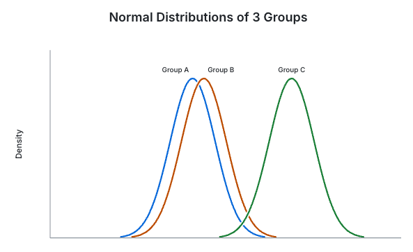
Now, we have 3 rating distributions and assume that they are normally distributed. Subjects mostly liked omelets with Roquefort cheese because they thought it was a heavy taste. They found the other two to be mild in taste and rated them close. We have three mean values: Mw, Mc, and Mr. We call the mean of the means the grand mean, Mg. We can say that if the distributions are close, then Mg will be close to the individual means, or vice versa.
By applying ANOVA, we are comparing between-group and within-group variability. Between-group variability refers to variations between the distributions of individual groups. Within-group variance refers to variations caused by differences within individual groups, as not all the values within each group are the same.
The idea behind ANOVA is quite intuitive. Even if all three types of cheese were equally popular, we wouldn’t expect every group to receive the same average rating. Some differences would occur simply because people have different preferences.
The important question is whether the differences between group averages are large compared to the natural variation within each group.
If the group averages are far apart while the ratings within each group are relatively consistent, we have stronger evidence that the population means are not all equal. However, if ratings vary greatly within each group, differences between group averages may reflect random variation.
This is exactly what ANOVA tries to distinguish.
F Statistic
The F ratio compares between-group variability with within-group variability. A larger F value indicates that differences between group means are large relative to within-group variation, providing stronger evidence against the null hypothesis.
A smaller F value indicates that the observed differences are relatively small compared to within-group variation. However, this does not necessarily mean that the population means are equal.
F = Between-group variability / Within-group variability
F = (SSB / dfb) / (SSW / dfw)
SSB: Between-group sum of squares; the sum of squared differences between each group mean (Mx) and the grand mean (Mg), weighted by the number of observations in each group.
SSW: Within-group sum of squares; the sum of squared differences between each observed value and its corresponding group mean (Mx).
dfb: Degrees of freedom between groups: 3 − 1 = 2
dfw: Degrees of freedom within groups: (19 − 1) + (19 − 1) + (19 − 1) = 54
19 is the number of observations in our example.
Before applying ANOVA, we should understand when its results can be trusted.
Classical one-way ANOVA relies on three main assumptions:
Independence: Observations should be independent of each other. For example, each participant should provide an independent rating, rather than having the same participant rate multiple omelets without accounting for repeated measurements.
Normality: The errors (residuals) within each group should be approximately normally distributed. ANOVA is reasonably robust to moderate departures from normality, especially with sufficiently large and balanced groups.
Equal variances: The population variances across groups should be approximately equal. If the variances differ substantially, Welch’s ANOVA may be more appropriate.
These assumptions matter because ANOVA’s statistical conclusions depend on how well the data match the conditions underlying the test.
For example, if the same customers rate all three omelets, their ratings are related. In that case, repeated-measures ANOVA may be more appropriate than ordinary one-way ANOVA.
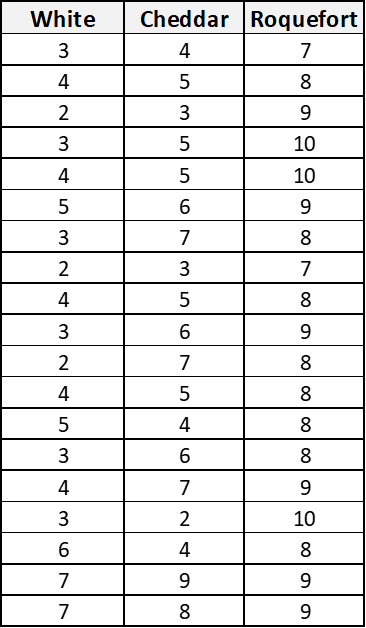
Now let’s calculate the ratio with the help of Python and dummy data by using one-way ANOVA. (We use one-way since there is only one independent variable).
Hypothesis
H0: There is no difference in means.
H1: At least one group is different.
Sum Squares
import pandas as pd df = pd.read_csv('dummy.csv') # Read dummy data and calculate meansMw, Mc, Mr = df.mean()[0], df.mean()[1], df.mean()[2] # Grand meanMg = (Mw + Mc + Mr) / 3Mw = 3.89, Mc = 5.32, Mr = 8.52
Mg = 5.91
# Within-group sum of squaresdf.loc[len(df), :] = Mw, Mc, Mrss_w = (((df.iloc[:-1] - df.iloc[-1])**2).sum()).sum() # Between-group sum of squaresss_b = ((df.shape[0] - 1) * (df.iloc[-1] - Mg)**2).sum()Within groups the sum of squares = 114.63, Between groups the sum of squares = 213.93
# F-Valuedfb = 2dfw = 54 F = (ss_b / dfb) / (ss_w / dfw)So the F-value is 50.39. We will decide whether to reject the null hypothesis by looking at the critical value in the F table. You can find the table here (opens in a new tab). Our critical value is approximately 3.17 (alpha taken as 0.05). Since our F-value is much higher than the critical value, we can reject the null hypothesis.
This means we have statistically significant evidence that at least one population mean differs from the others.
Rejecting the null hypothesis is an important result, but it doesn’t tell us everything.
Check the p-value
Instead of looking up critical values manually, we can also calculate the p-value using Python.
from scipy.stats import f p_value = f.sf(F, dfb, dfw)print(p_value)The p-value measures how unusual an F statistic at least this large would be if all population means were equal and the assumptions of the test held.
If the p-value is below our chosen significance level (typically 0.05), we reject the null hypothesis.
2. Find which groups are different
ANOVA only tells us that at least one population mean differs. It doesn’t tell us which cheese types are responsible for the difference.
For that, we can use a post-hoc test, such as Tukey’s HSD, which compares individual group means while accounting for multiple comparisons.
For example, we might find that roquefort is rated significantly higher than both white cheese and cheddar, while the difference between white cheese and cheddar is not statistically significant.
3. Consider practical significance
A statistically significant result doesn’t necessarily mean the difference matters in practice.
For example, suppose one cheese receives an average rating of 7.1 and another receives 7.2. With enough observations, even this small difference might be statistically significant. But would that justify switching ingredients, considering their costs and availability?
ANOVA helps us determine whether the observed differences provide evidence against equal population means. It doesn’t tell us whether those differences are important for our business decisions.
We can also examine an effect-size measure, such as eta-squared (η²), to understand how much of the observed variation in ratings is associated with the cheese groups.
Conclusion
When we look at the normal distribution graphs at the beginning of the article, we can easily see differences between the cheese groups. But in real cases, things will not be so clear and easy.
When the dependent variable is numerical and the independent variable is categorical, ANOVA allows us to test whether the group means differ beyond what we would expect from random variation.
The key idea is simple: ANOVA compares the differences between groups with the variation within those groups. If the differences between groups are sufficiently large, we have evidence that not all population means are equal.
However, a significant ANOVA result is only the beginning. We should also check whether the assumptions are reasonable, identify which groups differ, and consider whether those differences are meaningful in practice.
In our restaurant example, ANOVA can help us understand whether customers rate omelets differently depending on the cheese used. But choosing the best cheese also requires considering the size of those differences and other practical factors.
Now it’s time to have an omelet.
Check your understanding
Take a moment to revisit what you learned. Choose one answer for each question. Anonymous results help improve this article.
Key terms
| Term | What people say | What it actually means |
|---|---|---|
| One-way ANOVA | Comparing several averages | A statistical test of whether population means are equal across groups defined by one categorical independent variable. |
| Null hypothesis (H0) | The means are the same | The claim that all groups have equal population means; ANOVA assesses the evidence against this claim. |
| Grand mean | The overall average | The mean across all observations. With equal group sizes, it is also the average of the group means. |
| Between-group variability | How far apart the groups are | Variation between group means and the grand mean. The between-group sum of squares weights squared differences by group size. |
| Within-group variability | How much ratings vary inside a group | Variation of individual observations around their own group mean, summarized by the within-group sum of squares. |
| F-statistic | Between-group variation compared with within-group variation | The between-group mean square divided by the within-group mean square. Larger values provide stronger evidence against equal population means. |
| p-value | How unusual the result is | Assuming equal population means and the test’s assumptions, the probability of an F-statistic at least as large as the observed one. |
| Post-hoc test | Finding which groups differ | A follow-up comparison, such as Tukey’s HSD, that compares individual group means while accounting for multiple comparisons. |
| Practical significance | Does the difference matter? | Whether the size of a difference matters for the actual decision, considering factors such as ingredient costs and availability. |
Keep reading

Chi-Square Tests in Python: Goodness of Fit and Independence
Learn when to use chi-square goodness-of-fit and independence tests, calculate them in Python, and check assumptions with football and beer examples.

Chart.js with Django using Ajax
In this example, we will transfer data between Django and JavaScript and dynamically update a chart in the browser. We will use Chart.js to render the chart and jQuery's $.ajax()…