Chi-Square Tests in Python: Goodness of Fit and Independence
Learn to compare observed and expected counts through football, beer, and Python.

Chi-square tests help us answer questions about categorical data by comparing observed counts with the counts we would expect under a null hypothesis. For example, do football-team preferences match a claimed distribution? Is someone’s choice of beer associated with the team they support? We’ll explore these questions using two chi-square tests: the goodness-of-fit test and the test of independence.
The two tests answer different questions:
Goodness-of-fit test: Does the distribution of one categorical variable match specified proportions? For example, do observed football-team preferences match the proportions we expected?
Test of independence: Are two categorical variables associated? For example, is football-team preference associated with beer choice?
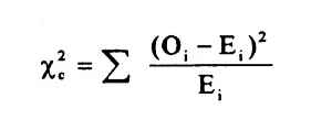
Both tests compare observed counts with expected counts under the null hypothesis. In the formula, Oᵢ is an observed count and Eᵢ is its corresponding expected count. For each category or table cell, we square the difference between these counts, divide by the expected count, and sum the results.
Larger chi-square values indicate greater disagreement between the observations and the null hypothesis. Whether that disagreement is statistically significant depends on the degrees of freedom and the chosen significance level. The subscript c in the image denotes the degrees of freedom; we’ll calculate these separately for each test.
Imagine that Swiss researchers claim that, among supporters of these three Istanbul clubs, 45% support Galatasaray, 35% support Fenerbahçe, and 20% support Beşiktaş. This is a fictional example, and we want to check whether our observations agree with those proportions.
We invite 100 people who support one of these clubs to join us for a beer in Taksim Square and ask which team they support. We record 54 Galatasaray supporters, 38 Fenerbahçe supporters, and 8 Beşiktaş supporters.
Under the claimed distribution, the expected counts are:
Galatasaray: 100 × 0.45 = 45
Fenerbahçe: 100 × 0.35 = 35
Beşiktaş: 100 × 0.20 = 20
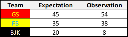
Our hypotheses are:
Null hypothesis (H₀): The population proportions are 45%, 35%, and 20%.
Alternative hypothesis (H₁): At least one population proportion differs from its specified value.
We choose a significance level of α = 0.05 before analysing the results. Each person should contribute one response, observations should be independent, and expected counts should be sufficiently large. All three expected counts here exceed the commonly used minimum of five.
Because there are three categories and the expected proportions were specified in advance, the degrees of freedom are:
df = k − 1 = 3 − 1 = 2
With the total fixed at 100, knowing two category counts determines the third.
Now we substitute the observed and expected counts into the formula.
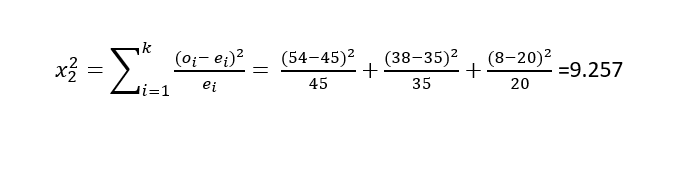
The resulting chi-square statistic is approximately 9.257. With two degrees of freedom and α = 0.05, the critical value is approximately 5.991.
Since 9.257 > 5.991, we reject the null hypothesis. The data provide evidence that the population proportions differ from the specified distribution, assuming the test’s sampling conditions hold.
We can calculate the statistic, p-value, and critical value with Python:
from scipy.stats import chi2, chisquare observed = [54, 38, 8]expected = [45, 35, 20] alpha = 0.05df = len(observed) - 1 result = chisquare(f_obs=observed, f_exp=expected)critical_value = chi2.ppf(1 - alpha, df=df) print(f"Chi-square statistic: {result.statistic:.3f}")print(f"Degrees of freedom: {df}")print(f"Critical value: {critical_value:.3f}")print(f"P-value: {result.pvalue:.4f}")Output:
Chi-square statistic: 9.257Degrees of freedom: 2Critical value: 5.991P-value: 0.0098The p-value is below 0.05, giving the same decision as the critical-value comparison.
Our Taksim example illustrates the calculation, but recruiting passersby over a beer would not establish a representative sample. We should therefore be cautious about extending its result to the wider population.
Let’s return to our 100 football supporters and add a second categorical variable: beer choice. We record one choice per person and ask whether it is associated with the team they support.
For this fictional example, we use two mutually exclusive categories: Pilsner and other lagers. Pilsner is itself a type of lager, so simply labelling the categories “Pilsner” and “Lager” would be ambiguous.

Our observed counts form a contingency table:
| Team | Pilsner | Other lagers | Total |
|---|---|---|---|
| Galatasaray | 34 | 20 | 54 |
| Fenerbahçe | 5 | 33 | 38 |
| Beşiktaş | 4 | 4 | 8 |
| Total | 43 | 57 | 100 |
Our hypotheses are:
Null hypothesis (H₀): Football-team preference and beer choice are independent in the population.
Alternative hypothesis (H₁): Football-team preference and beer choice are associated in the population.
Under independence, the expected count in each cell is:
Expected count = (row total × column total) / grand total
For example, the expected number of Galatasaray supporters choosing Pilsner is:
E = (54 × 43) / 100 = 23.22
Applying the same calculation to every cell gives:
| Team | Pilsner | Other lagers |
|---|---|---|
| Galatasaray | 23.22 | 30.78 |
| Fenerbahçe | 16.34 | 21.66 |
| Beşiktaş | 3.44 | 4.56 |
We use the same chi-square statistic as before, summing over all six cells. Keep the expected counts at full precision during calculation and round only the reported results.
The degrees of freedom are:
df = (rows − 1) × (columns − 1) = (3 − 1) × (2 − 1) = 2
The calculated statistic is χ² ≈ 22.747.
However, the expected counts for Beşiktaş are 3.44 and 4.56, both below five. This makes the usual chi-square approximation questionable. We’ll therefore check the result using a Monte Carlo test, which simulates contingency tables under independence while preserving the observed row and column totals.
The following code requires SciPy 1.15 or later:
from scipy.stats import chi2_contingency, MonteCarloMethod # Rows: Galatasaray, Fenerbahçe, Beşiktaş# Columns: Pilsner, other lagersobserved = [ [34, 20], [5, 33], [4, 4],] result = chi2_contingency(observed, correction=False) method = MonteCarloMethod(n_resamples=99_999)resampled = chi2_contingency( observed, correction=False, method=method,) print(f"Chi-square statistic: {result.statistic:.3f}")print(f"Degrees of freedom: {result.dof}")print("Expected counts:")print(result.expected_freq)print(f"Monte Carlo p-value: {resampled.pvalue:.6f}")The simulated p-value may vary between runs. In our checked run, it was approximately 0.000010, below the chosen significance level of 0.05.
We therefore reject the null hypothesis. Under the test’s sampling assumptions, the data provide evidence of an association between football-team preference and beer choice. This does not establish that supporting a particular team causes someone to choose a particular beer. The sampling limitations from our Taksim example still apply.
Chi-square tests compare observed counts with expected counts under a null hypothesis. Use a goodness-of-fit test to examine whether one categorical variable follows specified proportions. Use a test of independence to examine whether two categorical variables are associated.
Before applying either test, check that each observation contributes to one category or cell, observations are independent, and expected counts are sufficiently large for the chi-square approximation. When expected counts are small, consider a suitable alternative, such as the Monte Carlo approach used in our independence example.
A statistically significant result provides evidence against the null hypothesis under the test’s assumptions. Failing to reject the null does not establish that it is true. Likewise, an association does not establish causation, and a small p-value does not overcome limitations in how the sample was collected.
Check your understanding
Take a moment to revisit what you learned. Choose one answer for each question. Anonymous results help improve this article.
Key terms
| Term | What people say | What it actually means |
|---|---|---|
| Categorical variable | A label or group | A variable whose values identify categories, such as football team or beer choice. |
| Observed count | What we recorded | The number of observations actually recorded in a category or contingency-table cell. |
| Expected count | What the null hypothesis predicts | The count expected under the null hypothesis. For independence, it equals the row total multiplied by the column total, divided by the grand total. |
| Goodness-of-fit test | Do the proportions match? | A test of whether one categorical variable follows a specified distribution of proportions. |
| Test of independence | Are the variables associated? | A test of whether two categorical variables are independent in the population. |
| Null hypothesis (H₀) | The claim being tested | The specified proportions in a goodness-of-fit test, or independence between variables in a test of independence. |
| Alternative hypothesis (H₁) | What differs from the null | At least one specified proportion differs, or the two categorical variables are associated, depending on the test. |
| Chi-square statistic (χ²) | Observed versus expected disagreement | The sum, across categories or cells, of the squared difference between observed and expected counts divided by the expected count. |
| Degrees of freedom | How many counts can vary freely | For the examples in this article, k − 1 for goodness of fit with specified proportions, and (rows − 1) × (columns − 1) for independence. |
| Significance level (α) | The decision threshold | A threshold chosen before analysis for deciding whether to reject the null hypothesis. The examples use 0.05. |
| p-value | How unusual the result is under the null | Under the null hypothesis and test assumptions, the probability of a test statistic at least as extreme as the observed one. It is not the probability that the null hypothesis is true. |
| Contingency table | Counts grouped by two variables | A table whose cells contain counts for combinations of categories from two categorical variables. |
| Monte Carlo test | Checking significance through simulation | A test that estimates a p-value by simulating outcomes under the null hypothesis. The independence example preserves the observed row and column totals. |
Keep reading

ANOVA Test in Python
Analysis of variance (ANOVA) is a statistical method that determines whether there is a statistically significant difference between the means of at least three groups defined by a categorical independent variable, using a quantitative dependent variable.

Chart.js with Django using Ajax
In this example, we will transfer data between Django and JavaScript and dynamically update a chart in the browser. We will use Chart.js to render the chart and jQuery's $.ajax()…